
Seinfeld: The Tidytext Analysis
I began working on the basis of this post nearly two years ago, when I read an article analyzing how Seinfeld had changed over its seasons. At the time, I was still a student and thought using the scripts as data for a class project would be interesting. I got as far as beginning to crudely scrape the data, but realized I did not know where to begin as far as any analysis. So instead I did the project on something else, and left the Seinfeld data to gather figurative dust. More recently, I learned of the tidytext package and it’s excellent book, “Text Mining with R” by Julia Silge and David Robinson, and decided to continue the project.
The Data
Seinfeld ran for nine seasons from 1989 - 1998, with a total of 180 episodes. Often called “the show about nothing”, the series was about Jerry Seinfeld, and his day to day life with friends George Costanza, Elaine Benes, and Cosmo Kramer. Transcriptions of each of the episodes can be found on the fan site Seinology.com. I scraped all the scripts using the rvest package. The first thing to grab is the link to each episode.
library(tidyverse)
library(rvest)

links <- read_html("http://www.seinology.com/scripts-english.shtml") %>%
  html_nodes(".spacer2 td:nth-child(1) a") %>%
  html_attr("href") %>%
  data_frame() %>%
  select(url = 1) %>%
  filter(grepl("shtml", url) & !duplicated(url)) %>%
  mutate(full_url = paste0("http://www.seinology.com/", url))
I then wrote a function that takes the URL for an episode and pulls the necessary data. Unfortunately, as the scripts were submitted to the site by different fans there is no standard format, making the scraping a little trickier. By using a combination of regular expressions and other tools, we are able to pull the necessary information. The function gets the needed data and returns a data frame where each row is a line of dialogue with the following variables:
season: the season the episode airedepisode: the episode numbertitle: the title of the episodewriter: the writer(s) of the episodescene_num: the scene number of the spoken linescene: the episode and scene number togetherspeaker: the speaker of the lineline: the spoken line
All text that is non-spoken, such as any transcribed stage directions or descriptions of actions, is not included. I then used the function to pull the data for every URL in the links table. The resulting data can be downloaded here. Note that the scene number is not available for certain episodes as the transcriber for some scripts did not include any indication of scenes. 1 I compared scene numbers with the graph in the article mentioned above and got very similar results. I found a few differences, but as this post does not use scene numbers I did not bother further.
library(stringr)

# function to pull any script return necessary data
pull_script <- function(page_url){

  # read in the full script
  script <- read_html(page_url) %>%
    html_nodes(".spacer2 font") %>%
    html_text() %>%
    paste0(collapse = "\n") %>%
    str_replace_all("\\u0092", "'") %>%
    str_replace_all("\\u0085", "...")

  # get season number
  season <- str_extract(script, "(?i)(?<=season )\\d")

  # get episode number
  episode <- str_extract(page_url, "\\d+")

  # get episode title
  title <- str_extract(script, "(?<= - ).*")

  # get writer
  writer <- str_extract(script, "(?i)(?<=written by(:)?\\s).*")

  # get lines
  script_edit <- str_replace_all(script, "\t|\\(.*?\\)|\\[.*?\\]|NOTE:", "")

  # regex patterns for pulling speakers and lines
  line_regex <- "(?<=\n[A-Z]{1,20}(\\.)?(\\s{1,20})?([A-Z]{1,20})?:).*"

  speaker_regex <- "(?<=\n)[A-Z]+(\\.)?(\\s)?([A-Z]+)?(?=:)"

  lines <- unlist(str_extract_all(script_edit, line_regex))

  lines <- str_replace_all(lines, "\\u0092", "'")

  # get the scenes and the speaker
  if (str_detect(script, "INT\\.|EXT\\.") & episode != 69){

    script_df <- data_frame(
      text = unlist(str_split(script, "INT\\.|EXT\\.")),
      scene_num = 0:(length(text) - 1)
    ) %>%
      # remove episode information
      slice(-1) %>%
      mutate(text = str_replace_all(text, "\t|\\(.*?\\)|\\[.?\\]|NOTE:", ""),
             speaker = str_extract_all(text, speaker_regex)) %>%
      unnest(speaker)

  } else {

    script_df <- data_frame(
      text = unlist(str_split(script, "(?<=\n|\t)\\[.*?\\]|scene:")),
      scene_num = 0:max((length(text) - 1), 1)
    ) %>%
      # remove episode information
      slice(-1) %>%
      mutate(text = str_replace_all(text, "\t|\\(.*?\\)|\\[.?\\]|NOTE:", ""),
             speaker = str_extract_all(text, speaker_regex)) %>%
      unnest(speaker)

  }

  if (nrow(script_df) == length(lines)){

    dat <- script_df %>%
      transmute(season = season,
                episode = as.numeric(episode),
                title = title,
                writer = writer,
                scene_num,
                scene = paste0("e", episode, "s", scene_num),
                speaker,
                line = lines)
  } else {

    dat <- data_frame(
      season = season,
      episode = as.numeric(episode),
      title = title,
      writer = writer,
      scene_num = NA,
      scene = NA,
      speaker = unlist(str_extract_all(script_edit, speaker_regex)),
      line = lines
    )

  }
  dat
}

# run for all episodes
seinfeld <- lapply(links$full_url, pull_script) %>%
  bind_rows()

seinfeld <- seinfeld %>%
  mutate(episode = as.numeric(episode))

seinfeld$scene[seinfeld$episode %in% c(54, 121)] <- NA
seinfeld$scene_num[seinfeld$episode %in% c(54, 121)] <- NA
Analysis
Nearly all of the following analysis is adapted from the previously mentioned book, Text Mining with R. The book is available online and does a fantastic job introducing text analysis, and giving examples of text mining. This post uses some of the methods to begin to explore the dialogue of Seinfeld.
We start by comparing word frequencies of the different characters. This analysis will be focused on the four main characters and how they compare to everyone else. There are some things we have to fix in the data before we can begin. In the first episode, Kramer is called Kessler so we change this. We then create a new variable that lists the speaker if they are one of Jerry, George, Elaine, or Kramer, and lists Other for everyone else. The data also includes some lines that are blank due to the script reading something like “ELAINE: (chuckles)” so we remove any blank lines as well. We then convert the text into a tidy one word per row format, and remove any stop words using an anti_join. With our data in a tidy format, we can begin to compare word frequencies of the main characters. We use tools from dplyr and tidyr 2 to do this.
library(tidyverse)

seinfeld$speaker[seinfeld$speaker == "KESSLER"] <- "KRAMER"

# remove blank lines and create new variable
seinfeld <- seinfeld %>%
  filter(line != "" & !is.na(line)) %>%
  mutate(speaker2 = ifelse(
    speaker %in% c("JERRY", "GEORGE", "KRAMER", "ELAINE"),
    speaker, "OTHER"))

# tidy the data to one word per line, removing stop words
tidy_scripts <- seinfeld %>%
  unnest_tokens(word, line) %>%
  anti_join(stop_words)

# get counts for each word by character
frequency <- tidy_scripts %>%
  mutate(word = str_extract(word, "[a-z']+")) %>%
  count(speaker2, word) %>%
  group_by(speaker2) %>%
  mutate(proportion = n / sum(n)) %>%
  select(-n) %>%
  spread(speaker2, proportion) %>%
  gather(speaker, proportion, ELAINE:KRAMER)
We can now plot the frequencies and compare the characters. The graph displays each of the four main characters against all other characters. Words that are said at similar frequencies are found along the diagonal line. The words below the line are said more often by that character, and words said less often are above the line.
ggplot(frequency, aes(x = proportion, y = OTHER,
                      color = abs(OTHER - proportion))) +
  geom_abline(color = "gray31", lty = 2) +
  geom_jitter(alpha = .02, size = 2.5, width = .3, height = .3) +
  geom_text(aes(label = word), check_overlap = TRUE, vjust = 1.5, size = 4) +
  scale_x_log10(labels = percent_format()) +
  scale_y_log10(labels = percent_format()) +
  scale_color_gradient(limits = c(0, .001), low = "#6A6EC2", high = "gray75") +
  facet_wrap(~speaker, ncol = 2) +
  labs(y = "OTHER", x = NULL)  +
  theme(legend.position = "none")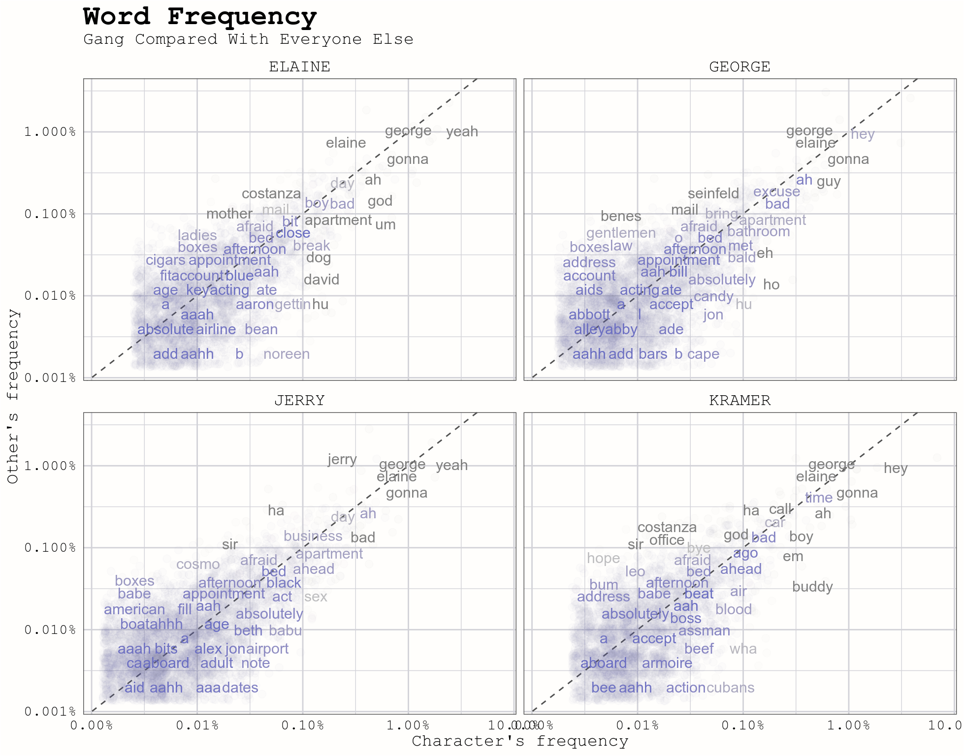
We learn that Elaine says “David” more than others, which makes sense as she dated David Puddy for number of episodes (and the rest of the gang normally called him “Puddy”). George says “Incredible” more than others, and Jerry says his own name less frequently than others. Some of my favorites are Kramer’s- he uses the words “buddy” and “assman” more frequently than anyone else.
We can use correlation tests to measure how similar the character’s word frequencies are. I’ve plotted the correlation, along with with a surrounding 95% interval, of each of the four leads compared with the word frequencies of all other characters combined.
frequency %>%
  group_by(speaker) %>%
  do(tidy(cor.test(.$proportion, .$OTHER))) %>%
  ggplot(aes(estimate, speaker)) +
  geom_errorbarh(aes(xmin = conf.low, xmax = conf.high, height = .2,
                     color = estimate), size = 1) +
  geom_point(color = "gray10", size=2) +
  labs(x = "correlation coefficient",
       title = "Correlation of Word Frequencies",
       subtitle = "Gang Compared With Everyone Else Combined") +
  theme(legend.position = "none",
        axis.title.y = element_blank())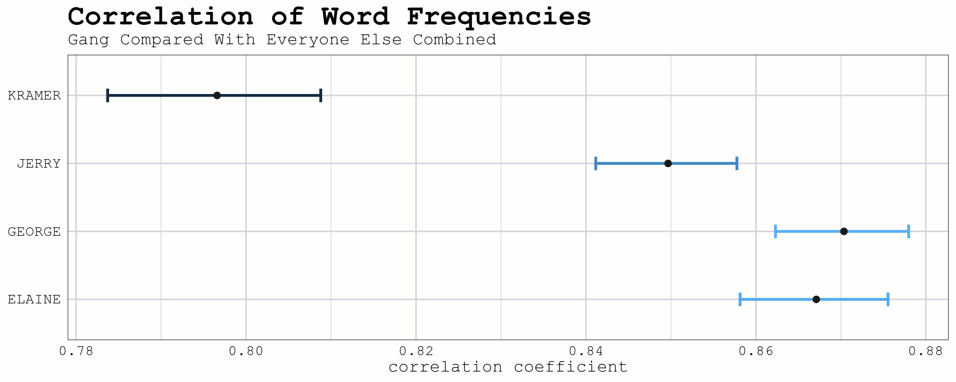
All four have fairly high correlation with the other characters, and are similar to one another. However, Kramer is less correlated than the others, meaning we now have evidence supporting the idea that Kramer is the most unique of the main characters!
Another statistic we can compute is tf-idf (term frequency - inverse document frequency). Tidy Text Mining says about tf-idf,
The statistic tf-idf is intended to measure how important a word is to a document in a collection (or corpus) of documents, for example, to one novel in a collection of novels or to one website in a collection of websites.
We use this to measure, and plot which words are most important for each character. Again, the tidytext package makes computing tf-idf fairly straighforward.
char_words <- seinfeld %>%
  unnest_tokens(word, line) %>%
  count(speaker2, word) %>%
  ungroup()

total_words <- char_words %>%
  group_by(speaker2) %>%
  summarize(total = sum(n))

char_words <- left_join(char_words, total_words) %>%
  bind_tf_idf(word, speaker2, n)

char_plot <- char_words %>%
  arrange(desc(tf_idf)) %>%
  mutate(word = factor(word, levels = rev(unique(word))))

char_plot %>%
  filter(speaker2 != "OTHER") %>%
  group_by(speaker2) %>%
  top_n(10) %>%
  ungroup() %>%
  ggplot(aes(word, tf_idf, fill = speaker2)) +
  geom_col(show.legend=FALSE) +
  facet_wrap(~speaker2, scales = "free") +
  coord_flip() +
  labs(x = "tf-idf",
       title = "Most Important Words by Character",
       subtitle = "Measured by tf-idf") +
  theme(legend.position = "none",
        axis.title.y = element_blank())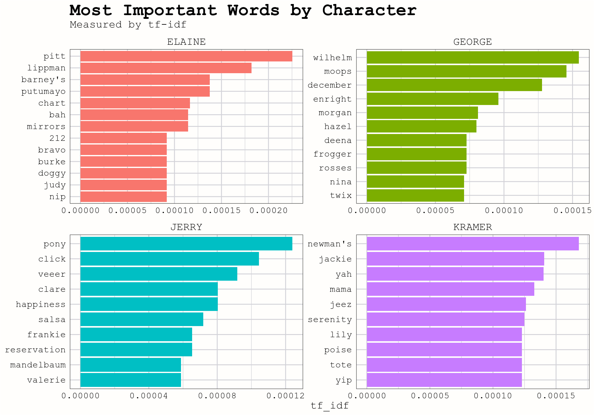
We can do the same thing, but instead calculate the most important word in each episode.
episode_words <- seinfeld %>%
  unnest_tokens(word, line) %>%
  count(episode, title, word, sort = TRUE) %>%
  ungroup()

total_words <- episode_words %>%
  group_by(episode, title) %>%
  summarize(total = sum(n))

episode_words <- left_join(episode_words, total_words) %>%
  bind_tf_idf(word, episode, n)

top_episodes <- episode_words %>%
  arrange(episode, desc(tf_idf)) %>%
  filter(!duplicated(episode)) %>%
  transmute(episode,
            title,
            word,
            n,
            total,
            tf_idf = round(tf_idf, 4))
Most important word in each episode
Many of the most important words can also be found in the title. There are also many episodes where character names unique to that episode are most important. Looking through the table we see other ones that can help us remember what happened in certain episodes.
Lastly, we can look at the network of words to see which words are most related with one another. First we tidy the data, but instead of having one word per row, this time we use two. We then separate the words into different columns, and filter out rows where either word is a stop word. We then use the igraph and ggraph packages to get the necessary information to make the graph.
library(igraph)
library(ggraph)

script_bigrams <- seinfeld %>%
  unnest_tokens(bigram, line, token = "ngrams", n = 2)

bigrams_sep <- script_bigrams %>%
  separate(bigram, c("word1", "word2"), sep = " ")

bigrams_filtered <- bigrams_sep %>%
  filter(!word1 %in% stop_words$word) %>%
  filter(!word2 %in% stop_words$word) %>%
  filter(word1 != word2)

bigram_counts <- bigrams_filtered %>%
  count(word1, word2, sort = TRUE)

bigram_graph <- bigram_counts %>%
  filter(n > 10) %>%
  graph_from_data_frame()

set.seed(10)

a <- grid::arrow(type = "closed", length = unit(.15, "inches"))

ggraph(bigram_graph, layout = "fr") +
  geom_edge_link(aes(edge_alpha = n), show.legend = FALSE,
                 arrow = a, end_cap = circle(.03, 'inches')) +
  geom_node_point(color = "lightblue", size = 3) +
  geom_node_text(aes(label = name), vjust = 1, hjust = 1) +
  theme_void()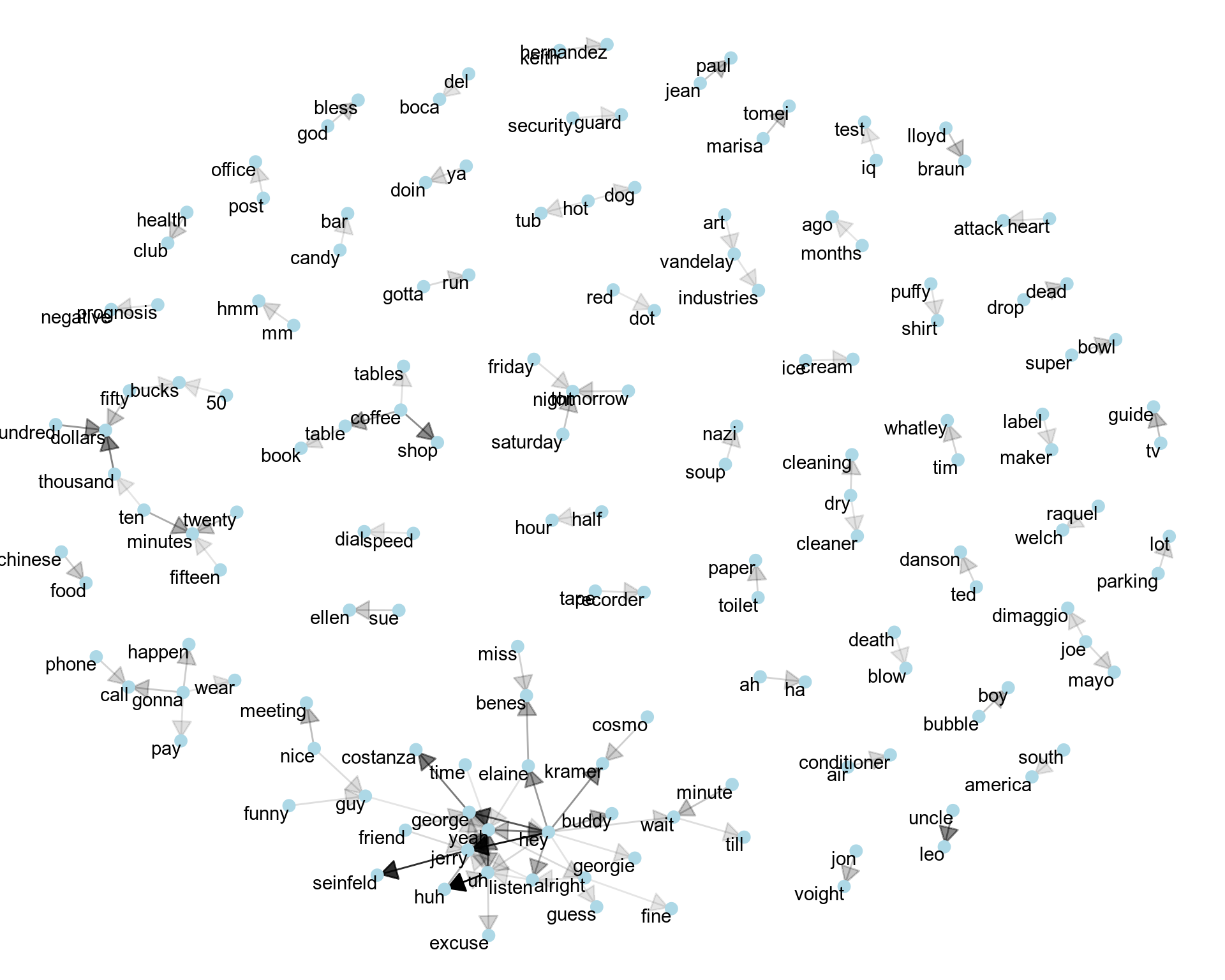
As we look at the network, there are some common word pairs: half hour, security guard, toilet paper, Chinese food, and others. We also see some phrases that are unique to the show, including: puffy shirt, bubble boy, soup nazi, prognosis negative, and Art Vandelay Industries
This is just the beginning of what is possible using tidy tools to analyze the scripts. In my next post, I’ll do some basic sentiment analysis to look see if the characters changed as the show went on- and to see if there any evidence of Independent George.